TurboWAVE Utilities¶

The turboWAVE utilities are contained in the python package twutils. If you followed the Easy Install guidance, you should already have twutils as part of your turboWAVE environment.

Apart from the installer and visualization components, twutils contains modules that are useful for pre and post processing.

Module `twutils.pre`¶

This module contains functions and classes to help with setting parameters for turboWAVE input files.

class pre.QuinticPulseData¶

Contains constants characterizing a quintic pulse with unit amplitude and base-to-base duration.

energy = integration over square of quintic pulse

FWHM = FWHM of square of quintic pulse

class pre.SimUnits(n1)¶

Contains constants characterizing plasma units. Class is created with the unit density in mks units.

t1 = unit of time in seconds

x1 = unit of length in meters

E1 = unit of electric field in volts per meter

pre.courant(dx, dy, dz, c=1.0)¶

Returns maximum time step allowed by the vacuum Courant condition.

Parameters:

dx (float) – cell size in x
dy (float) – cell size in y
dz (float) – cell size in z
c (float) – speed of light in the preferred units (defaults to plasma units)

Returns:

maximum time step

pre.getexp(a0, w0, r0, risetime, n1)¶

Get experimental pulse parameters from simulation parameters. Inputs are in plasma units, outputs in mks.

Parameters:

a0 (float) – vector potential
w0 (float) – angular frequency
r0 (float) – 1/e of amplitude radius
risetime (float) – quintic rise parameter
n1 (float) – unit density in mks units

Returns:

(intensity,power,energy,FWHM)

pre.getsim(U0, l0, r0, FWHM, n1)¶

Get simulation pulse parameters from experimental parameters. Inputs are in mks, outputs in plasma units.

Parameters:

U0 (float) – pulse energy
l0 (float) – central wavelength
r0 (float) – 1/e of amplitude radius
FWHM (float) – pulse length, full-width-half-maximum of intensity
n1 (float) – unit density

Returns:

(vector potential,angular frequency,quintic risetime)

pre.ncrit(wavelength)¶: Returns critical plasma density given a wavelength (mks units)

Module `twutils.QO.ionization`¶

This module can be used to compute ionization rates that may be needed in pre or post processing. It contains dictionaries of atomic data, and classes for computing ionization rates based on various models appearing in the literature. The ionization classes use atomic units, but include routines for converting to and from mks units.

References¶

The ionization models herein are detailed in the following references.

L.V. Keldysh, Sov. Phys. JETP 20 (5), 1307 (1965)
A.M. Perelemov, V.S. Popov, M.V. Terent’ev, Sov. Phys. JETP 23 (5), 924 (1966)
M.V. Ammosov, N.B. Delone, V.P. Krainov, Sov. Phys. JETP 64 (6), 1191 (1986)
G.L. Yudin and M.Y. Ivanov, Phys. Rev. A 64, 013409 (2001)
S.V. Popruzhenko, V.D. Mur, V.S. Popov, D. Bauer, Phys. Rev. Lett. 101, 193003 (2008)
M. Klaiber, E. Yakaboylu, K.Z. Hatsagortsyan, Phys. Rev. A 87, 023417 and 023418 (2013)

Constants¶

Dictionary ip: keys are atomic symbols (e.g. ‘H’,’He’,etc.), values are lists of ionization potentials in eV.
Dictionary atomic_mass: keys are atomic symbols, values are atomic masses in proton mass units.
Dictionary atomic_number : keys are atomic symbols, values are the number of protons.

An example of usage is as follows:

import twutils.QO.ionization as iz

print('argon ionization potential =',iz.ip['Ar'][0])
print('argon[3+] ionization potential =',iz.ip['Ar'][3])
print('atomic mass of argon is',iz.atomic_mass['Ar'])

Classes and functions¶

class ionization.ADK(averaging, Uion, Z, lstar=0, l=0, m=0)¶: Full ADK for arbitrary states

class ionization.ADK00(averaging, Uion, Z)¶: ADK theory simplified for lstar=l=m=0

class ionization.AtomicUnits¶

Class for converting to and from atomic units. Ionization classes derive from this.

energy_to_au(u)¶: Convert an energy in eV to atomic units

energy_to_eV(u)¶: Convert an energy from atomic units to eV

field_to_au(field)¶: Convert electric field from mks to atomic units

field_to_mks(field)¶: Convert electric field from atomic to mks units

length_to_au(x)¶: Convert a length from mks to atomic units

length_to_mks(x)¶: Convert a length from atomic to mks units

rate_to_au(rate)¶: Convert a time from mks to atomic units

rate_to_mks(rate)¶: Convert a time from atomic to mks units

time_to_au(t)¶: Convert a time from mks to atomic units

time_to_mks(t)¶: Convert a time from atomic to mks units

ionization.CycleAveragingFactor(Uion, E)¶

Returns the PPT cycle averaging factor, multiply static rate by this factor to get average rate.

Parameters:

Uion (double) – ionization potential in atomic units
E (double) – electric field in atomic units

class ionization.HybridTheories(averaging, Uion, Z, lstar=0, l=0, m=0, w0=0, terms=1)¶: Base class for theories that handle both multiphoton and tunneling limits

class ionization.Hydrogen(averaging, Uion, Z)¶: Landau & Lifshitz formula for hydrogen, using PPT averaging

class ionization.Ionization(averaging, Uion, Z, lstar=0, l=0, m=0, w0=0, terms=1)¶

Base class for computing ionization rates

ExtractEikonalForm(E, dt, w00=0.0, bandwidth=1.0)¶

Extract amplitude, phase, and center frequency from a carrier resolved field E. The assumed form is $E = \Re\{Ae^{i\phi}\}$ .

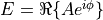Parameters:

E (numpy.array) – Electric field, any shape, axis 0 is time.
dt (double) – time step.
w00 (double) – Center frequency, if zero deduce from the data (default).
bandwidth (double) – relative bandwidth to keep, if unity no filtering (default).

Rate(Es)¶

Get the ionization rate, returned value is in atomic units. The object’s internal state decides whether this is a static or cycle averaged rate.

Parameters:: Es (np.array) – Time domain electric field in atomic units, any shape. If a complex envelope is given $|Es|$ is expected to give the crest.

ToAverage()¶: Switch to averaging. This must not be called more than once.

ToStatic()¶: Switch to static rate. This must not be called more than once.

class ionization.KYH(averaging, Uion, Z)¶: KYH theory for relativistic tunneling, using the dressed coulomb corrected SFA (Eq. 97)

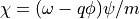
ionization.Keldysh_Parameter(omega, Uion, E)¶

Compute the adiabaticity parameter (Keldysh parameter)

Parameters:

omega (double) – radiation frequency in atomic units
Uion (double) – ionization potential in atomic units
E (double) – electric field in atomic units

Returns:

dimensionless adiabaticity parameter

class ionization.PMPB(averaging, Uion, Z, lstar=0, l=0, m=0, w0=0, terms=1)¶

PMBP theory, similar to PPT but with improved Coulomb factor, assuming m=0. Take lstar=0,l=0,m=0 to strictly recover PMPB Eq. 6.

Rate(Es)¶

Get the ionization rate, returned value is in atomic units. The object’s internal state decides whether this is a static or cycle averaged rate.

Parameters:: Es (np.array) – Time domain electric field in atomic units, any shape. If a complex envelope is given $|Es|$ is expected to give the crest.

class ionization.PPT(averaging, Uion, Z, lstar=0, l=0, m=0, w0=0, terms=1)¶

PPT theory accounting for multiphoton and tunneling limits, but assuming m=0. This is PPT Eq. 54 multiplied by the standard Coulomb factor, and taking m=0. For the bound state coefficient we use ADK Eq. 19. If static rate is requested, the result is only valid in the limit gamma=0

Rate(Es)¶

Get the ionization rate, returned value is in atomic units. The object’s internal state decides whether this is a static or cycle averaged rate.

Parameters:: Es (np.array) – Time domain electric field in atomic units, any shape. If a complex envelope is given $|Es|$ is expected to give the crest.

class ionization.PPT_Tunneling(averaging, Uion, Z, lstar=0, l=0, m=0)¶: Evaluating the PPT theory in the tunneling limit, with the infinite sum solved analytically. This is PPT Eq. 59 multiplied by the standard Coulomb factor, and taking gamma=0. For the bound state coefficient we use ADK Eq. 19.

ionization.Shifted_Uion_H(E)¶: Returns the Stark shifted ionization energy of Hydrogen

class ionization.YI(averaging, Uion, Z, lstar=0, l=0, m=0, w0=0, terms=1)¶

Yudin-Ivanov phase dependent ionization rate, Eq. 17., assuming m=0.

Rate(amp, phase)¶

Get the phase dependent rate. The Phase can be extracted using the Ionization class method ExtractEikonalForm.

Parameters:

amp (numpy.array) – Amplitude of the field, any shape
phase (numpy.array) – Phase of the field, any shape

Module `twutils.QO.stationary`¶

This module computes stationary states of numerical atoms. It can be used to generate state files for use with quantum optics modules.

Classes and functions¶

stationary.DiracEnergyLevel(cylindrical, Qnuc, qorb, morb, nr, jam, jzam, Bz, energy_estimate=0.99)¶

Returns Dirac energy levels indexed by nr,jam,jzam. Spherical stability of an electronic atom requires Z<=137. Cylindrical stability requires Z<=68.

Parameters:

cylindrical (boolean) – is this a cylincrical atom
Qnuc (float) – charge of the nucleus
qorb (float) – charge of the orbiting particle
morb (float) – mass of the orbiting particle
nr (int) – radial quantum number [0,1,2,…]
jam (float) – total angular momentum [0.5,1.5,2.5,…]
jzam (float) – total angular momentum projection [-jam,…,jam]
Bz (float) – magnetic field (must be weak)

stationary.DiracHypergeometricArgument(w, cylindrical, Qnuc, qorb, morb, nr, jam, jzam, Bz)¶

Auxilliary function used to find weak field energy levels. At present cylindrical only. Energy is the solution of f(w)==0.

Parameters:

w (float) – energy of the level, depending on usage possibly guess
cylindrical (boolean) – is this a cylincrical atom (currently must be true)
Qnuc (float) – charge of the nucleus
qorb (float) – charge of the orbiting particle
morb (float) – mass of the orbiting particle
nr (float) – radial quantum number
jam (float) – total angular momentum
jzam (float) – total angular momentum projection
Bz (float) – external magnetic field (must be weak)

stationary.DiracMatrix(cylindrical, grid, phi, qorb, morb, jam, lam, jzam, Bz)¶

Returns matrix of the discretized time-independent Dirac operator. For N grid points we obtain a 2Nx2N matrix corresponding to 2 components. The two components are $f$ and $g$ which in turn form the bispinor. See, e.g., Landau and Lifshitz QED section 35.

Parameters:

cylindrical (boolean) – is this a cylincrical atom
grid (array) – grid array, can get from SoftCorePotential function
phi (array) – potential array, can get from SoftCorePotential function
qorb (float) – charge of the orbiting particle
morb (float) – mass of the orbiting particle
jam (float) – total angular momentum [0.5,1.5,…], ignored in cylindrical case
lam (int) – parity number, must be jam $\pm 1/2$ , or in cylindrical case, jzam $\pm 1/2$
jzam (float) – total angular momentum projection [-jam,…,jam], or in cylindrical case, any half integer
Bz (float) – magnetic field (must be weak in spherical case)

stationary.KGEnergyLevel(cylindrical, Qnuc, qorb, morb, nr, lam, lzam, Bz)¶

Returns KG energy level indexed by nr,lam,lzam. Spherical stability of an electronic atom requires Z<=68. Cylindrical stability requires lam>0.

Parameters:

cylindrical (boolean) – is this a cylincrical atom
Qnuc (float) – charge of the nucleus
qorb (float) – charge of the orbiting particle
morb (float) – mass of the orbiting particle
nr (int) – radial quantum number [0,1,2,…]
lam (int) – orbital angular momentum [0,1,2,…]
lzam (int) – orbital angular momentum projection [-lam,…,lam]
Bz (float) – magnetic field (must be weak)

stationary.KGMatrix(cylindrical, grid, phi, qorb, morb, lam, lzam, Bz)¶

Returns matrix of the discretized time-independent KG operator. This uses the leapfrog friendly Hamiltonian representation. For N grid points we obtain a 2Nx2N matrix corresponding to 2 components. The second component is $\chi = (\omega-q\phi)\psi/m$

Parameters:

cylindrical (boolean) – is this a cylincrical atom
grid (array) – grid array, can get from SoftCorePotential function
phi (array) – potential array, can get from SoftCorePotential function
qorb (float) – charge of the orbiting particle
morb (float) – mass of the orbiting particle
lam (int) – orbital angular momentum [0,1,2,…], ignored in cylindrical case
lzam (int) – orbital angular momentum projection [-lam,…,lam], or any integer in cylindrical case
Bz (float) – magnetic field (must be weak in spherical case)

stationary.SchroedingerEnergyLevel(Qnuc, qorb, morb, nr, lam)¶

Returns Schroedinger energy levels indexed by nr and lam. The principle quantum number is nr+lam+1.

Parameters:

Qnuc (float) – charge of the nucleus
qorb (float) – charge of the orbiting particle
morb (float) – mass of the orbiting particle
nr (int) – radial quantum number [0,1,2,…]
lam (in) – orbital angular momentum [0,1,2,…]

stationary.SoftCorePotential(Qnuc, r0, num_pts, dr)¶

Create scalar potential on a radial grid

Parameters:

Qnuc (float) – charge of the nucleus
r0 (float) – soft core radius
num_pts (int) – number of interior grid points, total is num_pts+2
dr (float) – radial grid spacing

Returns:

an array of radial points and an array of potentials, including ghost cells

ReturnType:

tuple with the two arrays (grid,phi)

class stationary.StationaryStateTool(cylindrical, grid, phi, nr, jam, lam, jzam)¶

Class for managing stationary states, and creating state files

GetBaseComponents(energy_guess)¶

Gets 2 components used to form the wavefunction, call them f and g. For KG returns a Hamiltonian decomposition, with f the usual scalar, and g an auxiliary function. The Feshbach-Villars decomposition is then $(f+g)/\sqrt{2}$ , $(f-g)/\sqrt{2}$ . For Dirac returns f,g from L&L, which may be used to form the bispinor.

Parameters:: energy_guess (float) – initial guess of the energy
Returns:: En,f,g,sorted (En is the selected eigenvalue, sorted are the first few eigenvalues)

GetWavefunction(f, g)¶: Return 4 components (0,1,2,3) derived from the base components f and g. For KG only components 1 and 2 are relevant, components 0 and 3 may be ignored. For KG we return the simple decomposition with psi1 the usual scalar wavefunction. The Feshbach-Villars decomposition is then 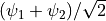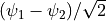$(\psi_1+\psi_2)/\sqrt{2}$ , $(\psi_1-\psi_2)/\sqrt{2}$ . For Dirac the 4 components are the radial part of the bispinor.

StandardFilename(Z)¶

Return a filename appropriate for the current quantum state

Parameters:: Z (float) – atomic number, purely for labeling
Returns:: string with the filename

WriteFile(file_name, psi0, psi1, psi2, psi3, En, softCoreRadius, Qnuc)¶: Write the state file given the current quantum state

__init__(cylindrical, grid, phi, nr, jam, lam, jzam)¶

Create a stationary state tool.

Parameters:

cylindrical (bool) – is this a cylindrical atom
grid (array) – radial grid, can be output from SoftCorePotential()
phi (array) – potential on the radial grid, can be output from SoftCorePotential()
nr (int) – radial quantum number [0,1,2,…] (cannot be 0 in certain cases)
jam (float) – see lower level functions for possible values
lam (int) – see lower level functions for possible values
jzam (float) – see lower level functions for possible values. This triggers Dirac or KG treatment depending on whether integer or half-integer.

__weakref__¶: list of weak references to the object

stationary.nu_to_MeV(energy)¶: take energy from natural units to MeV

stationary.nu_to_au(energy)¶: take energy from natural to atomic units

stationary.nu_to_eV(energy)¶: take energy from natural units to eV

stationary.nu_to_keV(energy)¶: take energy from natural units to keV

Module `twutils.NLO`¶

This module contains parameters for dielectric materials that can be used in turboWAVE, as well as functions to evaluate their numerical dispersion properties. This module uses mks units.

Classes and functions¶

class NLO.BBO¶: Contains parameters describing 2 oscillator model for BBO crystals

NLO.analyticDF(wa, kz, oscParams, n=1)¶

Returns analytical dispersion function (intended as argument to fsolve)

Parameters:

wa (array-like) – two-element array with real & imaginary part of angular frequency
kz (float) – real wavenumber
oscParams (class) – instance of an oscillator class defined in this module
n (int) – polarization axis numbered from 1-3

NLO.analyticWavenumber(w, oscParams, n=1)¶

Compute k(w) from analytical dispersion relation

Parameters:

w (float) – angular frequency [mks]
oscParams (class) – instance of an oscillator class defined in this module
n (int) – polarization axis numbered from 1-3

class NLO.fused_silica¶: Contains parameters describing 3 oscillator model for fused silica

class NLO.mag_fluoride¶: Contains parameters describing 3 oscillator model for magnesium fluoride

NLO.numericalDF(wa, kz, oscParams, dt, dz, n=1)¶

Returns numerical dispersion function (intended as argument to fsolve)

Parameters:

wa (array-like) – two-element array with real & imaginary part of angular frequency
kz (float) – real wavenumber
oscParams (class) – instance of an oscillator class defined in this module
dt (float) – timestep [mks]
dz (float) – cell size [mks]
n (int) – polarization axis numbered from 1-3

NLO.numericalWavenumber(w, oscParams, dt, dz, n=1)¶

Compute k(w) from numerical dispersion relation

Parameters:

w (float) – angular frequency [mks]
oscParams (class) – instance of an oscillator class defined in this module
dt (float) – timestep [mks]
dz (float) – cell size [mks]
n (int) – polarization axis numbered from 1-3

class NLO.silicon_carbide¶: Contains parameters describing 2 oscillator model for silicon carbide

class NLO.vacuum¶: Contains parameters describing vacuum

TurboWAVE Utilities¶

Module `twutils.pre`¶

Module `twutils.QO.ionization`¶

References¶

Constants¶

Classes and functions¶

Module `twutils.QO.stationary`¶

Classes and functions¶

Module `twutils.NLO`¶

Classes and functions¶

Table of Contents

Previous topic

Next topic

This Page

TurboWAVE Utilities¶

Module twutils.pre¶

Module twutils.QO.ionization¶

References¶

Constants¶

Classes and functions¶

Module twutils.QO.stationary¶

Classes and functions¶

Module twutils.NLO¶

Classes and functions¶

Module `twutils.pre`¶

Module `twutils.QO.ionization`¶

Module `twutils.QO.stationary`¶

Module `twutils.NLO`¶