Electromagnetic Wave Modes
Electromagnetic wave modes are are monochromatic, continuous wave solutions of Maxwell’s equations. TurboWAVE makes use of such solutions to inject radiation into the simulation. Since the analytical expressions are typically approximate in some way, turboWAVE numerically forces the initial or boundary fields into compliance with Maxwell’s divergence equations. The total solution is then guaranteed to satisfy Maxwell’s equations, to within a discretization error.
The initial or boundary fields are always derived from a vector potential in the Coulomb gauge, regardless of the field solver that is used. It follows that  is automatically satisfied (divergence of a curl is identically zero). During initialization, an elliptical solver is used to guarantee
  . The elliptical solver is also used to generate electrostatic fields in case there is a charge separation in the initial condition.
Coordinates
A point in Cartesian coordinates is denoted

A point in cylindrical coordinates is denoted

A point in spherical coordinates is denoted

Note that the azimuthal variable is always  . The polar angle is
  .
.
Phase and Envelope Functions
All the modes considered here are in the form

where A is some component of the vector potential (not necessarily Cartesian), T is a pulse envelope function, and  is a phase function that may have a complex spatial dependence. The argument of the pulse function,
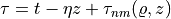
  , can also have a complex spatial dependence. The envelope and phase function arguments are typically closely related. To express this fact, the phase is always put in the form
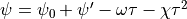
Here  is the center frequency of the wave,
  is the
 chirp parameter, and  is a reference phase set by the user independently for each wave in the system. The anomalous phase term
  allows for arbitrary modifications to the relationship between the phase and amplitude contours.
In general, all functions may depend on the refractive index,  .
.
The pulse envelope factor T is put into the monochromatic solution by hand, and will generally introduce an error, except in the eikonal limit. Since the divergence error is corrected numerically, the factor T introduces no error into the overall solution, in cases where a Maxwell field solver is used to advance the fields in time.
Tip
The origin of space and time are set by the user through the wave parameters focus position, delay and risetime. The coordinate system can also be rotated arbitrarily.
Note
Normalized units are used in the following.
Plane Wave
For a plane wave we have the constant amplitude

and the pulse function argument

with no anomalous phase.
Bessel Beams
The Bessel beam modes are exact Maxwell solutions that are separable in cylindrical coordinates. As of this writing, only the lowest order is supported:
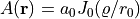
The pulse and phase variables are the same as for a plane wave.
Hermite Gaussian
The Hermite-Gaussian modes are paraxial beam modes that are separable in Cartesian coordinates. The amplitude and pulse function argument are in the forms


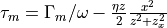
where m and n are the mode numbers along the x and y axes. The anomalous phase term is twice the Guoy phase

The factor of two reverses the sign of an equal and opposite Guoy phase that is put in the envelope function to make it subluminal in the confocal region.
For the x direction mode factors:
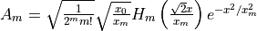
where

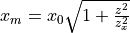
Here the inputs are the index of refraction , the waist radius  , and the peak vector potential
  . The factors for the y direction are exactly analogous.
Laguerre Gaussian
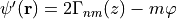
The Laguerre-Gaussian modes are paraxial beam modes that are separable in cylindrical coordinates. The amplitude factor and pulse function argument are in the forms
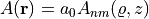
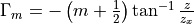
where n and m are the radial and azimuthal mode numbers. The anomalous phase is
As in the Hermite case the factor of two multiplying the Guoy phase compensates for a reverse Guoy phase in the pulse function argument. The radial factors are:

where


Here the inputs are the index of refraction , the waist radius  , and the peak vector potential .
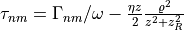
Multipole Fields
The multipole fields are exact Maxwell solutions that are separable in spherical coordinates. They are also the states of definite angular momentum of the photon. As of this writing, only the lowest order magnetic multipole (dipole) is supported. Multipole radiation is most compactly expressed as a standing wave. For a magnetic multipole of any order we have
where  is the appropriate vector spherical harmonic function, and
  is the spherical Bessel function. The spherical Bessel function is real valued and carries the rapidly varying spatial dependence.
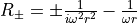
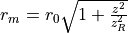
For a magnetic dipole field, it is straightforward to decompose the Bessel function into incoming and outgoing waves, which allows the field to be put in the standard form above. The two solutions are:

Here  is the coordinate of the first maximum of the spherical Bessel function, and