Input File: Tools¶

General Information¶

TurboWAVE objects come in two flavors, Modules and Tools (not to be confused with post-processing tools). Modules are the high level objects that orchestrate a simulation. Tools (internally called ComputeTool objects) are lower level objects dedicated to specific computations. Tools are intended to be attached to one or more modules (modules can share the same tool). Modules can be placed in a hierarchy. Tools can only be attached to a module.

Tools are created like any object, see Input File: Base.

Many modules are able to create their tools automatically. This page emphasizes those that tend to benefit from explicit management by the user.

Radiation Injection¶

To inject radiation, you specify a type of electromagnetic mode, directives defining its particular parameters, and attach it to a field solver. For an in depth description of the available radiation modes see Electromagnetic Wave Modes. If the wave starts inside the box, an elliptical solver may be used to refine the initial divergence. If the wave starts outside the box, it will be coupled in, provided the field solver supports this. Each wave object has its own basis vectors $({\bf u},{\bf v},{\bf w})$ , with ${\bf u}$ the electric field polarization direction and ${\bf w}$ the propagation direction. All the available modes respond to the same set of directives. These are as follows:

new <key> [<name>] [for <module_name>] { <directives> }

Parameters:

key (str) – The key determines the type of mode. Valid keys are plane wave, hermite gauss, laguerre gauss, bessel beam, airy disc, and multipole.
module_name (str) – Name given to a previously defined field solver module.
directives (block) –
The following directives are supported:
direction = ( nx , ny, nz )
Parameters:
nx (float) – first component of ${\bf w}$ in standard basis.

ny (float) – second component of ${\bf w}$ in standard basis.

nz (float) – third component of ${\bf w}$ in standard basis.
a = ( ax , ay , az )
If the peak vector potential is $a_0$ , then ${\bf a} = a_0{\bf u}$ . TurboWAVE will force transversality by making the replacement ${\bf a} \rightarrow {\bf w}\times{\bf a}\times{\bf w}$
Parameters:
ax (float) – first component of ${\bf a}$ in standard basis

ay (float) – second component of ${\bf a}$ in standard basis

az (float) – third component of ${\bf a}$ in standard basis
focus position = ( fx , fy , fz )
Parameters:
fx (float) – first focal position coordinate in standard basis

fy (float) – second focal position coordinate in standard basis

fz (float) – third focal position coordinate in standard basis
w = w0

Parameters:

w0 (float) – central frequency of the wave

refractiveindex = n0

Parameters:

n0 (float) – refractive index in the starting medium

chirp = x

Parameters:

x (float) – Multiply the amplitude by $\exp (-i\chi t^2)$ , with time referenced so that the center frequency occurs at the end of the risetime. Up-chirp results from $\chi>0$ . If you are trying to model the pulse from a grating compressor you may prefer to use a spectral phase.

spectral phase = { c2 , c3 , c4 , ... }

Multiplies the pulse spectrum by $\exp(i\varphi)$ , where $\varphi$ is given by a Taylor expansion about the center frequency. N.b. that applying this filter will change the pulse metrics. Up-chirp results from $c_2>0$ .

Parameters:

cn (float) – derivatives of the spectral phase, $c_n = \partial^n_\omega \varphi(\omega)$ . Note that c0 and c1 are not used, since the effects would be redundant.

sample points = sp

The number of points in the look-up table representing the pulse. Use this to better resolve complex spectral phases, or if you need to resolve the rising part of a near top-hat profile.

Parameters:

sp (float) – the number of sample points, defaults to 1024.

phase = p0

Parameters:

p0 (float) – phase shift in radians

delay = t0

Parameters:

t0 (float) – Front of wave reaches focus position after this amount of time

risetime = t1

holdtime = t2

falltime = t3
r0 = ( u0 , v0 )
Parameters:
u0 (float) – spot size at the vacuum waist in the ${\bf u}$ direction. Note this is not necessarily the spot size in the first coordinate of the standard basis. Spot size is measured at $1/e$ point of the field amplitude.

v0 (float) – spot size in the ${\bf v}$ direction.
mode = ( mu , mv )
Transverse mode numbers, different meanings depending on the mode type.
Parameters:
mu (int) – mode number in the ${\bf u}$ direction

mv (int) – mode number in the ${\bf v}$ direction
exponent = ( m , n )
This directive applies only to the paraxial beam modes, Hermite and Laguerre.
Parameters:
m (int) – exponent to use in transverse profile, default is 2 (standard Gaussian). If even induces order m supergaussian, if odd induces order m+1 cosine.

n (int) – If the mode is Hermite then n applies to the v-direction. If it is Laguerre then n is ignored.
shape = pulse_shape

Parameters:

pulse_shape (enum) – determines the shape of the pulse envelope, can be quintic (default), sin2, sech
boost = (gbx,gby,gbz)
Ask turboWAVE to transform the wave into the boosted frame. The parameters describing the wave should all be given in lab frame coordinates. The grid coordinates are taken as the boosted frame. At present this feature should only be used for paraxial modes propagating along the z-axis.
Parameters:
gbx (float) – component of 4-velocity in x-direction

gby (float) – component of 4-velocity in y-direction

gbz (float) – component of 4-velocity in z-direction
zones = z

Parameters:

z (int) – create a superposition of transversely periodic modes across z zones in each dimension. The number of zones should be odd, and large enough to span several spot sizes. This is useful for boosted frame simulations where the Rayleigh length is much shorter than the pulse duration.

Note

In the past there was a distinction between carrier resolved and enveloped radiation injection objects. This distinction has been retired. Envelope treatment is triggered automatically by attaching any radiation injection object to a enveloped field solver.

Matter Loading¶

The loading of matter into the simulation box is done using generate blocks. These take the same form whether we are loading particles or fluid elements. In loading matter it is important to distinguish the clipping region from the profile:

clipping region¶: A clipping region is a filter that multiplies a physical quantity by zero outside the region, and unity inside.
profile¶: A profile is a spatial distribution of some intrinsic parameter such as density.

Note

Our definition of thermal velocity is 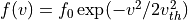$f(v) = f_0\exp(-v^2/2v_{th}^2)$

Note

For isotropic distributions we have $kT = mv_{th}^2$ , $v_i^{rms} = v_{th}$ , and $v_{tot}^{rms} = \sqrt{3}v_{th}$ .

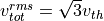Matter Loading Transformations¶

The way profiles are defined, positioned, and oriented, is analogous to the way regions are. In particular, there is a native position and orientation that is modified by applying a set of transformations. See Input File: Geometry for an explanation of the transformations that can be applied.

Matter Loading Shared Directives¶

In addition to the geometry transformations, the following directives may be used with any profile type

clipping region = name

Load the matter only within the specified geometric region. See Input File: Geometry for documentation on creating complex geometric regions.

Parameters:: name (str) – the name of the geometric region to use

temperature = T

Parameters:: T (float) – initial temperature of the matter

thermal momentum = (pthx,pthy,pthz)

drift momentum = (px,py,pz)

loading = lmethod

Parameters:: lmethod (enum) – loading method. takes values deterministic, statistical

particle weight = wscheme

Parameters:: wscheme (enum) – takes values variable, fixed

type = profile_type

Matter loading encompasses mass, energy, and momentum. The type of profile determines which quantity is loaded.

Parameters:: profile_type (enum) – takes values density, energy, px, py, pz

timing = timing_type

Parameters:: timing_type (enum) – takes values triggered or maintained (default = triggered). Triggered profiles are additive. Maintained profiles try to hold fixed conditions.

t0 = start_time

Parameters:: start_time (float) – time at which matter loading begins.

t1 = stop_time

Parameters:: stop_time (float) – time at which matter loading ends. If timing is triggered this is ignored.

Specific Matter Loading Profiles¶

generate uniform <name> { <directives> }

Generate uniform density within the clipping region.

Parameters:

name (str) – name of module defining type of matter to load.
directives (block) –
The following directives are supported:

Shared directives: see Matter Loading Shared Directives

density = n0

Parameters:

n0 (float) – density to load

generate piecewise <name> { <directives> }

Generate piecewise varying density within the clipping region. The total density is the product of 4 piecewise functions:

$n(t,x,y,z) = T(t)X(x)Y(y)Z(z)$

Parameters:

name (str) – name of module defining type of matter to load.
directives (block) –
The following directives are supported:

Shared directives: see Matter Loading Shared Directives

tpoints = t_list

Parameters:

x_list (list) – Variable length list of floating point numbers giving the points at which $T(t)$ is known, e.g., { 0 , 1.5 , 3.4 , 5.1 }.

xpoints = x_list

Parameters:

x_list (list) – Variable length list of floating point numbers giving the points at which $X(x)$ is known, e.g., { 0 , 1.5 , 3.4 , 5.1 }.

ypoints = y_list

Parameters:

y_list (list) – Variable length list of floating point numbers giving the points at which $Y(y)$ is known, e.g., { 0 , 1.5 , 3.4 , 5.1 }.

zpoints = z_list

Parameters:

z_list (list) – Variable length list of floating point numbers giving the points at which $X(x)$ is known, e.g., { 0 , 1.5 , 3.4 , 5.1 }.

tdensity = td_list

Parameters:

td_list (list) – Variable length list of floating point numbers giving the values of $T(t)$ at the points listed with tpoints.

xdensity = xd_list

Parameters:

xd_list (list) – Variable length list of floating point numbers giving the values of $X(x)$ at the points listed with xpoints.

ydensity = yd_list

Parameters:

yd_list (list) – Variable length list of floating point numbers giving the values of $Y(y)$ at the points listed with ypoints.

zdensity = zd_list

Parameters:

zd_list (list) – Variable length list of floating point numbers giving the values of $Z(z)$ at the points listed with zpoints.

shape = my_shape

Parameters:

my_shape (enum) – quintic, quartic, triangle

symmetry = sym

Parameters:

sym (enum) – none, cylindrical, spherical. If cylindrical, x-profile is interpreted as radial, z-profile is axial, y is only used to define origin. If spherical, x-profile is radial, y and z are used only to define the origin.

mode number = nx ny nz

Multiply final profile by $\left[\cos(n_x x/2)\cos(n_y y/2)\cos(n_z z/2)\right]^2$

generate channel <name> { <directives> }

Generate density channel within the clipping region. The defining formula is

$n(x,y,z) = Z(z)\left(n_0 + n_2\rho^2 + n_4\rho^4 + n_6\rho^6\right)$

$\rho = \sqrt{x^2 + y^2}$

The matched beam condition for spot size $\rho_0$ is

$n_2 = 1/\pi r_e \rho_0^4$

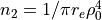
where $r_e$ is the classical electron radius, $n_0$ is arbitrary, and higher terms vanish. The normalization is

$n_i \rightarrow \frac{n_i}{n} \left(\frac{c}{\omega}\right)^i$

where $\omega$ is the unit frequency and $n$ is the unit density. This leads to the matched beam condition in normalized units as

$n_2 = 4/\rho_0^4$

Parameters:

name (str) – name of module defining type of matter to load.
directives (block) –
The following directives are supported:

Shared directives:
see Matter Loading Shared Directives

piecewise profile $Z(z)$ function

piecewise profile shape directive.
coefficients = n0 n2 n4 n6
Parameters:
n0 (float) – see $n_0$ in defining formula

n2 (float) – see $n_2$ in defining formula

n4 (float) – see $n_4$ in defining formula

n6 (float) – see $n_6$ in defining formula

generate column <name> { <directives> }

Generate density column within the clipping region.

$n(t,x,y,z) = Z(z)\exp(-t^2/\sigma_t^2 - x^2/\sigma_x^2 - y^2/\sigma_y^2)$

Parameters:

name (str) – name of module defining type of matter to load.
directives (block) –
The following directives are supported:

Shared directives:
see Matter Loading Shared Directives

piecewise profile $Z(z)$ function

piecewise profile shape directive.
size = ( sx , sy , sz )
Parameters:
st (float) – $\sigma_t$ in defining formula.

sx (float) – radius of column, per $\sigma_x$ in defining formula.

sy (float) – radius of column, per $\sigma_y$ in defining formula.

sz (float) – ignored.

generate gaussian <name> { <directives> }

Generate a Gaussian ellipsoid within the clipping region.

$n(t,x,y,z) = n_0 \exp(-t^2/\sigma_t^2 - x^2/\sigma_x^2 - y^2/\sigma_y^2 - z^2/\sigma_z^2)$

Parameters:

name (str) – name of module defining type of matter to load.
directives (block) –
The following directives are supported:

Shared directives: see Matter Loading Shared Directives

density = n0

Parameters:

n0 (float) – peak density, per defining formula.
size = ( st, sx , sy , sz )
Parameters:
st (float) – $\sigma_t$ in defining formula.

sx (float) – $\sigma_x$ in defining formula.

sy (float) – $\sigma_y$ in defining formula.

sz (float) – $\sigma_x$ in defining formula.

Conducting Regions¶

Conducting regions serve the following purposes:

Perfect conductors filling arbitrary cells in electromagnetic simulations

Antenna objects in electromagnetic simulations

Impermeable objects filling arbitrary cells in hydrodynamic simulations

Fixed potential objects filling arbitrary cells in electrostatic simulations

Fixed temperature objects filling arbitrary cells in hydrodynamic simulations

new conductor [<name>] [for <module_name>] { <directives> }

The electrostatic potential can be fixed within the conductor as

$\Phi(t) = \Phi_0 S(t) \cos(\omega t + \varphi)$

The dipole radiator elements oscillate according to

${\bf P}(t,x,y,z) = {\bf P}_0 S[T(t,x,y)] \sin[\omega T(t,x,y) + \varphi + {\bf k}_s \cdot {\bf r}]$

$T(t,x,y) = t + \frac{x^2+y^2}{2f}$

Parameters:

name (str) – Name given to the conductor
directives (block) –
The following directives are supported:

Shared directives:
Temporal envelope $S(t)$ is derived from pulse shape parameters per wave object

clipping region = name

Rotation of clipping region also rotates current distribution

Parameters:

name (str) – name of geometric region to use

temperature = T

Parameters:

T (float) – The temperature of the conductor can be fixed at T, serving as a dirichlet boundary condition for heat equations. Note that parabolic solver tools default to a homogeneous neumann condition (no heat flow).

enable electrostatic = tst

Parameters:

tst (bool) – this conductor will fix the potential

enable electromagnetic = tst

Parameters:

tst (bool) – this conductor will reflect EM waves

ANTENNA DIRECTIVES: Currents are driven with dipole oscillators. This avoids problems with static field generation. All the lists must be of equal length. Each list element is an oscillator. The total current is the superposition of the current of each oscillator.

current type = curr_typ

Parameters:

curr_typ (enum) – takes values electric, magnetic, or none

potential = lst

Determines $\Phi_0$ for each oscillator.

Parameters:

lst (list) – variable length list of scalar potentials, e.g., { 1.0 , 2.0 }

px = lst1 , py = lst2 , pz = lst3

Determines ${\bf P}_0$ for each oscillator.

w = w0

Determines $\omega$ for each oscillator.

phase = p0

Determines $\varphi$ for each oscillator.

f = f0

Parameters:

f0 (float) – Determines $f$ parameter that appears in $T(t,x,y)$ . This is supposed to produce a focus at the corresponding distance from the antenna (default = infinity).

ks = ksx ksy ksz

Apply linear phase variation to create tilted wave (default = 0).

gaussian size = ( sx , sy , sz )

Apply a gaussian spatial weight to the oscillator amplitudes.

Particle Movers¶

Particle movers are used with Species modules. As of this writing, there are no adjustable parameters.

There are three types of distinctions among mover tools:

Physics - differing physics models can call for differing mover tools

Dimensionality - optimization for an ignorable y-coordinate, or fully 3D

Algorithm - different discretization schemes

The Species module will automatically choose a mover if none is specified. It does this by looking at the grid, and the data that has been shared by other modules, and deducing the correct dimensionality and physics. The way the discretization scheme is selected favors legacy methods, at present.

Boris Mover¶

new boris mover [<name>] [for <module_name>] { <directives> }

This is the long-standing, standard, relativistic, electromagnetic mover. This is used by default if an electromagnetic field is detected, and there are no quantum or enveloped fields.

This mover is also selected if there is an electrostatic field solver. The electrostatic solver must provide the magnetic field, but may set it to zero.

There are no directives.

Higuera-Cary Mover¶

new hc mover [<name>] [for <module_name>] { <directives> }

This is a variation on the Boris mover that uses an estimate for the energy at the half-step that is thought to be more accurate. This is never chosen by default.

There are no directives.

PGC Mover¶

new pgc mover [<name>] [for <module_name>] { <directives> }

This is an extension of the Boris mover to account for the ponderomotive guiding center approximation. This is chosen if an enveloped field solver is detected.

There are no directives.

Unitary Mover¶

new unitary mover [<name>] [for <module_name>] { <directives> }

This is an alternative to the Boris mover, which is believed to be more accurate for ultra-relativistic parameters. This is never chosen by default.

There are no directives.

Bohmian Mover¶

new bohmian mover [<name>] [for <module_name>] { <directives> }: This moves particles using the Bohmian guidance condition. This is used to create Bohmian trajectories with the quantum optics modules. It is created automatically if a quantum propagator is detected.

Elliptic Solvers¶

All elliptic solvers share the following directives:

<coord>boundary = ( <bc1> , <bc2> )

Parameters:

coord (enum) – can be x, y, z
bc1 (enum) – boundary condition on lower side, can be open, dirichlet, neumann.
bc2 (enum) – boundary condition on lower side, can be open, dirichlet, neumann.

Inhomogeneous boundary conditions are implemented by using conductor tools to fix the potential. For external boundaries, the conductor must occupy the far ghost cells.

Iterative Solver¶

new iterative elliptic [<name>] [for <module_name>] { <directives> }

Uses successive over-relaxation to iteratively solve the elliptic equation. This solver is slow, but flexible. There is no limit on the topology of the boundary conditions, and arbitrary coordinates are supported. The following directives are supported:

Shared directives: see base elliptic solver

tolerance = <tol>

Parameters:

tol (float) – iterate until the residual is reduced to this level

overrelaxation = <ov>

Parameters:

ov (float) – overrides the default overrelaxation parameter (not generally recommended)

FACR Solver¶

new facr elliptic [<name>] [for <module_name>] { <directives> }: Uses Fourier analysis is in the transverse directions. This solver is fast, but boundary conditions can only be imposed on constant z-surfaces, and Cartesian coordinates are required. The following directives are supported:

Shared directives: see base elliptic solver

Eigenmode Solver¶

new eigenmode elliptic [<name>] [for <module_name>] { <directives> }

Uses generalized spectral resolution of the transverse coordinates. This solver works in arbitrary coordinates, and is fast as long as the transverse modes are truncated. Boundary conditions can only be imposed on constant z-surfaces. The following directives are supported:

Shared directives: see base elliptic solver

modes = <N>

Parameters:

N (int) – The number of transverse modes to keep. The modes are taken from an ordered list, sorted by magnitude of the eigenvalue.

Laser Propagator¶

Forward Propagator¶

new forward propagator [<name>] [for <module_name>] { <directives> }: This is an accurate propagator, but the axial integration is serial.

PhotoIonization¶

Ionization Shared Directives¶

All the photoionization tools support the following directives:

ionization potential = ip

Parameters:: ip (float) – Ionization potential, units are specified as usual, e.g., ionization potential = 13.6 [eV]

saturated rate = sr

Parameters:: sr (float) – saturate the ionization rate at this value

protons = np

Parameters:: np (int) – number of protons in nucleus (not needed for mpi model ; currently used to form residual charge only)

electrons = ne

Parameters:: ne (int) – number of bound electrons (not needed for mpi model ; currently used to form residual charge only)

ion species = is_name

Parameters:: is_name (str) – name of a species to add a particle to upon ionization (usually positive charge)

electron species = es_name

Parameters:: es_name (str) – name of a species to add a particle to upon ionization (usually negative charge)

Multi-photon Ionization¶

Model appropriate for low fields or high frequencies.

new multiphoton ionization [<name>] [for <module_name>] { <directives> }

The following directives are supported:

Shared directives: see above

reference field = E0

Parameters:

E0 (float) – $E_0$ , where the MPI rate is proportional to $(E/E_0)^{2l}$

ADK Tunneling Ionization¶

Model appropriate for high fields or low frequencies, and arbitrary atomic states.

new adk ionization [<name>] [for <module_name>] { <directives> }

The following directives are supported:

Shared directives: see above

orbital number = l

Parameters:

l (int) – the orbital quantum number of the state

orbital projection = m

Parameters:

m (int) – the projection of the orbital quantum number in the direction of the field

effective orbital number = lstar

Parameters:

lstar (float) – effective orbital quantum number

PPT Tunneling Ionization¶

This model evaluates the general PPT formula in the tunneling limit. Differs from ADK only in that the gamma function in the bound state coefficient is not approximated.

new ppt tunneling [<name>] [for <module_name>] { <directives> }

The following directives are supported:

Shared directives: see above

orbital number = l

Parameters:

l (int) – the orbital quantum number of the state

orbital projection = m

Parameters:

m (int) – the projection of the orbital quantum number in the direction of the field

effective orbital number = lstar

Parameters:

lstar (float) – effective orbital quantum number

KYH Tunneling Ionization¶

Model appropriate for high fields or low frequencies, based on a Coulomb corrected strong field approximation, and with relativistic corrections.

new kyh ionization [<name>] [for <module_name>] { <directives> }: The following directives are supported:

Shared directives: see above

PPT Photoionization¶

Cycle-averaged model that works across multi-photon and tunneling regimes (convergence in tunneling regime is slow). Assumes the projection of the orbital angular momentum in the direction of the field vanishes. Cannot be used for ionization due to carrier-resolved fields, i.e., must be used with an enveloped field solver.

new ppt ionization [<name>] [for <module_name>] { <directives> }

The following directives are supported:

Shared directives: see above

orbital number = l

Parameters:

l (int) – the orbital quantum number of the state

effective orbital number = lstar

Parameters:

lstar (float) – effective orbital quantum number

terms = n

Parameters:

n (int) – number of terms to keep in the PPT expansion.

PMPB Photoionization¶

Similar to the PPT model, except the Coulomb correction is improved in the multiphoton limit. In the original paper the orbital and effective orbital numbers are set to zero.

new pmpb ionization [<name>] [for <module_name>] { <directives> }

The following directives are supported:

Shared directives: see above

orbital number = l

Parameters:

l (int) – the orbital quantum number of the state

effective orbital number = lstar

Parameters:

lstar (float) – effective orbital quantum number

terms = n

Parameters:

n (int) – number of terms to keep in the PPT expansion.

Equation of State Tools¶

Equation of State (EOS) models are needed for hydrodynamics simulation. EOS models are encapsulated in tool objects that can be attached to appropriate modules in the usual way.

new eos ideal gas tool [<name>] [for <module_name>] { <directives> }: Directs a module to use the ideal gas equation of state. No directives.

new eos hot electrons [<name>] [for <module_name>] { <directives> }: Directs a module to use the ideal gas equation of state along with Braginskii electron transport coefficients. No directives.

new eos simple mie gruneisen [<name>] [for <module_name>] { <directives> }

Directs a module to use the simplified mie-gruneisen equation of state. The following directives are supported:

gruneisen parameter = grun

Parameters:

grun (float) – the gruneisen parameter relating density, temperature, and pressure

new eos linear mie gruneisen [<name>] [for <module_name>] { <directives> }

Directs a module to use the linear Hugoniot-based mie-gruneisen equation of state.

The following directives are supported:

gruneisen parameter = grun

Parameters:

grun (float) – the gruneisen parameter relating density, temperature, and pressure

reference density = nref

Parameters:

nref (float) – the reference density for the Hugoniot data

hugoniot intercept = c0

Parameters:

c0 (float) – y-intercept of the Hugoniot curve, typically the speed of sound

hugoniot slope = s1

Parameters:

s1 (float) – slope of the Hugoniot curve at the reference density

Diagnostics¶

Note

If a diagnostic tool is not explicitly attached to any module, it will be automatically attached to all modules. This is an optimization based on the observation that one would often like a similar type of output from all modules.

Diagnostic Formats¶

TurboWAVE binaries are in numerical Python (numpy) format (extension .npy). All metadata is in the file tw_metadata.json. Text files are generally tab delimited tables of ASCII data, with a one-line header containing column labels.

Box diagnostics produce a .npy file containing a four-dimensional array with axes (t,x,y,z). Phase space diagnostics write a similar array, but the axes can have different meanings. The grid data is found by looking up the 'grid' key. This returns a string with the name of the grid file containing the mesh point and time level information:

t = <t0>
axis1 = <x1> <x2> ... <xN>
axis2 = <y1> <y2> ... <yN>
axis3 = <z1> <z2> ... <zN>
<...more frames>

For static grids, the additional frames only have the line giving the elapsed time.

The orbit diagnostic produces a .npy file containing the detailed particle information:

Particle record 1 at time level 1
Particle record 2 at time level 1
...more particle records at time level 1
Particle record N at time level 1
Time level separator
Particle record 1 at time level 2
Particle record 2 at time level 2
...more particle records at time level 2
Particle record M at time level 2
...more time level separators and particle records

Each particle record is an 8 element vector (x,px,y,py,z,pz,aux1,aux2). The order of the particles within a time level is not significant. Particles must be identified by unique values of aux1 and aux2. The time level separator is a record with all zeros. Valid particles can never have aux1 = aux2 = 0.

Example Post-processing Script¶

Typical Python post-processing scripts begin like this:

import numpy as np
import json
import pathlib

my_path = pathlib.Path.home() / 'Run'
# Get a field component into a 4D numpy array with shape (t,x,y,z)
Ex = np.load(my_path / 'Ex.npy')
# Load the metadata into a dictionary (all metadata)
with open(my_path / 'tw_metadata.json','r') as f:
        meta = json.load(f)
# As an example of metadata, get the conversion factor to mks units.
# Note axis mapping, 0=t, 1=x, 2=y, 3=z, 4=data
mks_factor = meta['Ex.npy']['axes']['4']['mks multiplier']
# Get the name of the grid file
grid_file_name = meta['Ex.npy']['grid']

The grid data is a text file. One way to read it is with the following function:

def get_mesh_pts(grid_file_path,dims):
    """Try to find a grid warp file matching the npy file.
    If the file is found return [tmesh,xmesh,ymesh,zmesh].
    Each element is a list of the mesh points along the given axis.
    If the file is not found return unit length uniform mesh.
    Arguments: grid_file_path = pathlike, name of grid file.
               dims = expected shape of the data"""
    try:
        ans = [[],[],[],[]]
        with open(grid_file_path) as f:
            for line in f:
                l = line.split(' ')
                if l[0]=='t':
                    ans[0] += [float(l[-1])]
                if l[0]=='axis1' and len(ans[1])==0:
                    ans[1] = [float(x) for x in l[2:]]
                if l[0]=='axis2' and len(ans[2])==0:
                    ans[2] = [float(x) for x in l[2:]]
                if l[0]=='axis3' and len(ans[3])==0:
                    ans[3] = [float(x) for x in l[2:]]
        if len(ans[0])==dims[0] and len(ans[1])==dims[1] and len(ans[2])==dims[2] and len(ans[3])==dims[3]:
            return [np.array(ans[0]),np.array(ans[1]),np.array(ans[2]),np.array(ans[3])]
        else:
            warnings.warn('Grid file found but wrong dimensions ('+grid_file_path+').')
            return [np.linspace(0.0,1.0,dims[i]) for i in range(4)]
    except FileNotFoundError:
        warnings.warn('No grid file found ('+grid_file_path+').')
    except PermissionError:
        warnings.warn('Ignoring grid file ('+grid_file_path+') due to permissions.')
    return [np.linspace(0.0,1.0,dims[i]) for i in range(4)]

Diagnostics Shared Directives¶

The following directives may be used with any diagnostic

filename = f

Parameters:: f (str) – name of the file to write. Actual file names may be prepended with the name of some subset of the overall data associated with the diagnostic (some diagnostics write multiple files). This may be postpended with a filename extension such as .txt or .npy. The special name full causes the files to have only the prepended string and the extension in their names. This is the default.

clipping region = name

write data only within the specified geometric region. See Input File: Geometry for documentation on creating complex geometric regions. For some diagnostics there is a restriction on the complexity of the region.

Parameters:: name (str) – the name of the geometric region to use

t0 = start_time

Parameters:: start_time (float) – time at which diagnostic write-out begins (default=0).

t1 = stop_time

Parameters:: stop_time (float) – time after which diagnostic write-out ends (default=infinity).

period = steps

Parameters:: steps (int) – number of simulation cycles between write-outs.

time period = duration

Parameters:: duration (float) – simulated time between write-outs, overrides period if specified. If an adaptive time step is in use, this can approximate uniform spacing of write-outs.

galilean velocity = (vx,vy,vz)

Transform output to a Galilean frame, i.e., ${\bf r}' = {\bf r} - {\bf v}t$ . This transformation can be combined with a boosted frame.

Parameters:

vx (float) – x-component of the galilean transformation velocity
vy (float) – y-component of the galilean transformation velocity
vz (float) – z-component of the galilean transformation velocity

boost = (gbx,gby,gbz)

This is a request to unboost data generated in a boosted frame. As of this writing it is only implemented for orbit and phase space diagnostics, and there are some limitations (see below).

Parameters:

gbx (float) – component of 4-velocity in x-direction
gby (float) – component of 4-velocity in y-direction
gbz (float) – component of 4-velocity in z-direction

Specific Diagnostics¶

new box diagnostic [<name>] [for <module_name>] { <directives> }

Write out grid data as sequence of frames. Clipping region must be a simple box. This diagnostic produces several files per module, by default.

Parameters:

directives (block) –

The following directives are supported:

Shared directives: see Diagnostics Shared Directives

average = tst

Parameters:: tst (bool) – average over sub-grid, or not. If not, diagnose lower corner cell only.

skip = ( sx , sy , sz )

Defines a reduced grid produced by downsampling the full grid. The reduction factor is the product of the three skipping parameters. Note the centroid of the sampling points is shifted.

Parameters:

sx (int) – advance this many cells in the x-direction between writes
sy (int) – advance this many cells in the y-direction between writes
sz (int) – advance this many cells in the z-direction between writes

reports = { <fields> }

Parameters:: fields (list) – Put a list of fields to get restricted output. If omitted then all available fields are written.

new energy diagnostic [<name>] [for <module_name>] { <directives> }

Diagnostic of volume integrated quantities. Normalization includes the unit of particle number.

Parameters:

directives (block) –

The following directives are supported:

Shared directives: see Diagnostics Shared Directives

precision = digits

Parameters:: digits (int) – number of digits used to represent each result

new point diagnostic [<name>] [for <module_name>] { <directives> }

Diagnostic to write out grid data at a specific point.

Parameters:

directives (block) –

The following directives are supported:

Shared directives: see Diagnostics Shared Directives

point = (Px,Py,Pz): Coordinates of the point to diagnose. This is subject to the Galilean transformation (see Diagnostics Shared Directives).

new phase space diagnostic [<name>] [for <module_name>] { <directives> }

Diagnostic to write out up to 3D phase space projections. Setting a dimension to 1 produces a lower dimensional projection. The boost parameter can be used to put the data in the lab frame. It is important to note that if this is done, the frame write-out index still slices time in the boosted frame. On the other hand, explicit time axes are properly transformed.

Parameters:

species_name (str) – the name of the species to diagnose
directives (block) –
The following directives are supported:

Shared directives: see Diagnostics Shared Directives
axes = (ax1,ax2,ax3)
Determines the axes of the phase space. Axes can be any of t, x, y, z, mass, px, py, pz, g, gbx, gby, gbz. If a dimension collapses to 1, the axis is ignored, but still must be specified.
Parameters:
ax1 (enum) – the phase space variable to associate with axis 1

ax2 (enum) – the phase space variable to associate with axis 2

ax3 (enum) – the phase space variable to associate with axis 3
dimensions = (N1,N2,N3)
Parameters:
N1 (int) – cells along axis 1

N2 (int) – cells along axis 2

N3 (int) – cells along axis 3
bounds = (x0,x1,y0,y1,z0,z1)
Boundaries of the interrogation region. In boosted frame simulations, these can be specified in the lab frame by setting boost.
Parameters:
x0 (float) – lower bound for axis 1

x1 (float) – upper bound for axis 1

y0 (float) – lower bound for axis 2

y1 (float) – upper bound for axis 2

z0 (float) – lower bound for axis 3

z1 (float) – upper bound for axis 3
accumulate = acc

Parameters:

acc (bool) – if true the phase space data accumulates, otherwise write-out frames are resolved (default=false). This is especially useful for boosted frames.

new orbit diagnostic [<name>] [for <module_name>]

Diagnostic to write out full phase space data of the particles. In boosted frame simulations, data can be put in the lab frame by setting boost. Note however that the time separators in the data file lose their meaning in this case.

Caution

Orbit diagnostics can create excessively large files if not used carefully. To avoid this, define a species with a small number of test particles and use this on them.

Parameters:

species_name (str) – the name of the species to diagnose
directives (block) –
The following directives are supported:

Shared directives: see Diagnostics Shared Directives

minimum gamma = gmin

Parameters:

gmin (float) – only save data for particles with gamma greater than this. In boosted frame simulations, this can be specified in the lab frame by setting boost.

Input File: Tools¶

General Information¶

Radiation Injection¶

Matter Loading¶

Matter Loading Transformations¶

Matter Loading Shared Directives¶

Specific Matter Loading Profiles¶

Conducting Regions¶

Particle Movers¶

Boris Mover¶

Higuera-Cary Mover¶

PGC Mover¶

Unitary Mover¶

Bohmian Mover¶

Elliptic Solvers¶

Iterative Solver¶

FACR Solver¶

Eigenmode Solver¶

Laser Propagator¶

Forward Propagator¶

PhotoIonization¶

Ionization Shared Directives¶

Multi-photon Ionization¶

ADK Tunneling Ionization¶

PPT Tunneling Ionization¶

KYH Tunneling Ionization¶

PPT Photoionization¶

PMPB Photoionization¶

Equation of State Tools¶

Diagnostics¶

Diagnostic Formats¶

Example Post-processing Script¶

Diagnostics Shared Directives¶

Specific Diagnostics¶

Table of Contents

Previous topic

Next topic

This Page