Input Files
Everything about a turboWAVE simulation is determined by the input file. The input file can have any name, though it is best to not use spaces. The .tw extension can be made to trigger syntax highlights in certain editors. If no input file name is specified turboWAVE assumes it is stdin.
The turboWAVE input file is written in what amounts to a “little language”, which is described further in Input File: Base. Fortunately this language is very simple and does not impose a significant learning curve.
Dimensional Numbers
The turboWAVE parser comprehends units and dimensions. To write a dimensional number, simply add a postfix. As an example, enter 10 [ps] to indicate a value of 10 picoseconds. For the full list of available conversions see Specifying Units.
Normalized Plasma Units
Although turboWAVE’s internal comprehension of units insulates the user from the necessity of understanding normalizations, it is useful to appreciate their significance. TurboWAVE supports three normalization systems: natural units, atomic units, and plasma units. Plasma units are discussed here. Natural and atomic units are in Quantum Optics Modules.
The plasma normalization is motivated by the observation that any solution of the Vlasov equation can be scaled up or down to produce a family of solutions. We may as well express all quantities in a way that does not commit to which particular member of the family we are talking about. No particular scale is any better than another.
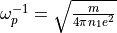
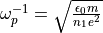
On the other hand, if an atomic process like ionization comes into the problem, then we must commit to a definite physical scale. For this reason, turboWAVE input files allow you to specify a unit of density that fixes the physical scale. Once this is chosen, to normalize some quantity given in physical units, divide by the unit given in Table I.
Quantity |
Unit |
cgs Symbol |
mks Symbol |
|---|---|---|---|
Number Density |
user specified |
|
|
Velocity |
speed of light |
c |
c |
Charge |
electronic charge |
e |
e |
Mass |
electronic mass |
m |
m |
Time |
derived |
|
|
Space |
derived |
|
|
Energy |
derived |
|
|
Momentum |
derived |
|
|
Scalar Potential |
derived |
|
|
Vector Potential |
derived |
|
|
Electric Field |
derived |
|
|
Magnetic Field |
derived |
|
|
Particle Number |
derived |
|
|


Tip
If you have a particular radiation frequency that is of interest, setting the unit of density to the critical density for that radiation will make the radiation angular frequency unity in simulation units.
Tip
You can make the unit of length correspond to a conventional unit by choosing the unit of density such that  comes out to your chosen unit (e.g., 1 cm). You can do something similar with the unit of time. However, the unit of time and space cannot both be nice decimal numbers in conventional units, since the speed of light is not.
On the Unit of Particle Number
One thing that can be confusing in the normalization scheme is that the unit of density is not connected to the unit of length in the expected way. This comes about because we are simultaneously demanding that the speed of light be unity, and that the unit of time be connected with the density. This can lead to erroneous normalization of certain quantities with a density buried in them. As an example, take current density. The naive construction might be to take the unit as  (wrong). The correct construction is
  .
.
It can be useful to identify, in this connection, a unit of particle number, per Table I. Take the unit of energy. The normalization in table I refers to the energy of a real particle “within” a simulation macroparticle. If we want the energy contained in the whole macroparticle, we must multiply by the unit of particle number. In fact, any volume integrated energy that turboWAVE writes out must include this factor if you want to convert to conventional units.
TurboWAVE Example Files
You will learn the most by studying the examples. They can be found in turboWAVE/core/examples and are organized into several directories. These are as follows.
hydro: Contains examples of hydrodynamic simulations that use the SPARC module. If you plan to use turboWAVE for hydro simulations, you should especially understand the simple-shock examples, and the diffusion example. The shock cases can be compared with an analytical theory. There is a Mathematica notebook in the folder which can be used to explore the analytical solution.pic: Contains examples of fully explicit PIC simulations. This contains especially variants on laser driven wakefields.pgc: Similar to thepicdirectory, except uses the ponderomotive guiding center approximation to model the laser fields.fluid: Cold relativistic fluid approximation for laser wakefield and beatwave cases.nonlinear-optics: Contains examples of the nonlinear optics model for laser radiation in crystals.quantum: Contains examples of atomic level processes using the quantum optoelectronics modules.misc: Some other examples.
TurboWAVE Reference
Detailed exposition of the input file elements are in the reference pages. Highlights include:
Input File: Base describes the input file “little language”
Input File: Tools describes some important tools that can be used in various modules
Input File: PIC describes modules used for PIC simulations
Input File: Fluids describes modules used for fluid simulations